 The determinant and the permanent of a matrix are central characters in an endeavour to bring the powerful weapons of modern geometry to a battle in the epic war of computer science: the P vs. NP problem.
JM Landsberg has recently written a wonderful introduction to geometric complexity theory which is how the corresponding research field is called. This has inspired me to borrow some of it and write about the permanent and the determinant of a matrix.
In linear algebra, the determinant is a value associated to each square matrix. It has many particularly nice properties and interpretations. For example, it can help to decide whether a system of linear equations represented by the matrix has a unique solution and it computes the volume of the parallelepiped spanned by its rows. For an 


The sum is taken over all permutations 


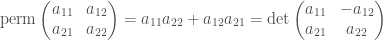
At a first glance, the permanent looks like a simplification of the determinant because it is given by essentially the same formula without the sign function:

The permanent is very useful because it can be employed to find the answer to counting problems like finding the number of perfect matchings in a bipartite graph. However, where the determinant can be computed in polynomial time, e.g. by Gaussian elimination, computing the permanent is #P-hard.
Now, in the case of two by two matrices, the determinant can be used to compute the permanent:
For larger matrices, however, computing the permanent by a determinant of the same size whose entries are given by linear forms of the entries of the original matrix is not possible. Then how about using the determinant of a matrix of a larger size? We would like to find a way to do this using determinants which are not too much larger. But the hardness result on computing the permanent means that using determinants with a size polynomial in the size of the matrix is winning the battle. A much more humble question is to find a representation using exponential size.
Bruno Grenet shows how to do this with an 
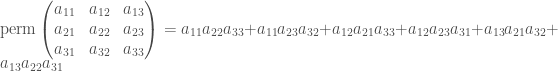
Let’s start with a three by three matrix:
In order to find a determinant representation for this permanent, we construct a graph from the subsets of the set 

The graph of subsets of the set
This graph is constructed in a way such that the vertices (the subsets) are grouped by size such that all sets of the same cardinality form one layer of the graph. I will refer to the layer containing sets of cardinality 


We can now order the vertices (for example as indicated by the red numbers in the figure) and represent the graph by its adjacency matrix:

This matrix has entry zero at position 
Now we can compute the determinant of this matrix and find that it is exactly the permanent of our matrix. You can use WolframAlpha to show that its determinant is indeed equal to the permanent. Why this is true is somewhat harder to see. It has to do with counting the number of cycle covers of the above graph. I invite you to have a look at the paper for more information.
